Build a Binary Classification Model

Target: Is the delivery “Late” (1) or “On Time” (0)?

Before using complex algorithms, we need a baseline model to compare against. A simple baseline is the “Majority Class” classifier, which always predicts the most frequent outcome.

Why? If 90% of deliveries are on time, a model with 90% accuracy might actually be doing nothing more than guessing “on time” every time. We have checked this baseline in the previous section and found that the majority class is “Delayed” at around 58%. So, our baseline model would predict “Delayed” for every delivery, giving us an accuracy of about 58%.

Install and Import Libraries¶

Required packages

You will need scikit-learn, xgboost, and plotnine to run the code in this notebook. You can install them using pip or conda:

Using pip:

pip install scikit-learn xgboost plotnine

Using conda:

conda install -c conda-forge scikit-learn py-xgboost plotnine

import pandas as pd
import numpy as np

from sklearn.model_selection import train_test_split
from sklearn.preprocessing import LabelEncoder
from sklearn.metrics import (
    classification_report,
    confusion_matrix,
    roc_auc_score,
    accuracy_score,
)

import xgboost
from xgboost import XGBClassifier

Check XGBoost version.

print(f"xgboost version: {xgboost.__version__}")

xgboost version: 3.2.0

Load Data¶

df = pd.read_csv(
    "http://raw.githubusercontent.com/bdi593/datasets/main/amazon-on-time-delivery-data/on-time-delivery-data.csv"
)
df

Loading...

Preprocess Data for Modeling¶

Select Features and Target¶

X = df.drop(columns=["classification_ontime"])
y = df["classification_ontime"]

Encode Target Variable to Integer¶

le = LabelEncoder()
y = le.fit_transform(y)

print(dict(zip(le.classes_, le.transform(le.classes_))))

{'Delayed': np.int64(0), 'On time': np.int64(1)}

Split Data into Train and Test Sets¶

The random_state parameter ensures that the split is reproducible, meaning you will get the same train and test sets every time you run the code. This is important for consistency when evaluating model performance. 42 is a commonly used value for random_state, but you can choose any integer.

X_train, X_test, y_train, y_test = train_test_split(
    X, y, test_size=0.2, random_state=42, stratify=y
)

The Inputs¶

X: Your feature matrix (independent variables).
- Example: zipcode, total_items,
y: Your target variable (dependent variable).
- "classification_ontime"

The Arguments¶

test_size=0.2: 20% of the data goes into the test set, and the remaining 80% goes into the training set
- Since we have 45,000 rows, this means:
  - 36,000 rows for training
  - 9,000 rows for testing
random_state=42: Controls randomness.
- Ensures the split is reproducible
- If someone else runs this code with random_state=42, they get the same split
- The number 42 is arbitrary (it’s just a seed), although it’s a popular choice in the data science community.
stratify=y: Ensures that the class distribution in the train and test sets is the same as in the original dataset.
- Example: If your original dataset has:
  - 70% class 0
  - 30% class 1
- Then both training and test sets will also have:
  - 70% class 0
  - 30% class 1
- Without stratification, you might get an imbalanced split.
- ⚠️ Only use stratify=y for classification tasks (not regression).

Outputs¶

The function returns 4 objects:

Variable	Meaning
`X_train`	Features for training
`X_test`	Features for testing
`y_train`	Labels for training
`y_test`	Labels for testing

Build Classifier¶

xgb_model = XGBClassifier(
    n_estimators=300,
    learning_rate=0.05,
    max_depth=4,
    subsample=0.8,
    colsample_bytree=0.8,
    objective="binary:logistic",
    eval_metric="logloss",
    random_state=42,
)

xgb_model.fit(X_train, y_train)

Loading...

Model Arguments (Parameters)¶

The arguments you pass when creating the XGBoost model are called hyperparameters. They control how the model learns from the data. Choosing the right hyperparameters can significantly affect your model’s performance.

Parameter	Type	What It Controls	Effect on Model	Typical Range / Notes
`n_estimators`	int	Number of boosting rounds (trees)	More trees → more complex model; can reduce bias but increase overfitting	100-1000 common
`learning_rate`	float	Step size shrinkage after each tree	Smaller values → slower learning, usually better generalization (needs more trees)	0.01-0.3
`max_depth`	int	Maximum depth of each tree	Deeper trees → capture more complex patterns but risk overfitting	3-10 typical
`subsample`	float	Fraction of training samples used per tree	<1.0 adds randomness → reduces overfitting	0.5-1.0
`colsample_bytree`	float	Fraction of features used per tree	Adds feature randomness → reduces overfitting	0.5-1.0
`objective`	string	Loss function being optimized	Determines type of task (binary, multi-class, regression)	`"binary:logistic"` for binary classification
`eval_metric`	string	Metric used to evaluate model performance during training	Does not affect training directly, just monitoring	`"logloss"`, `"auc"`, `"error"` common
`random_state`	int	Seed for reproducibility	Ensures same random sampling each run	Any fixed integer

Check Model Performance¶

After training the XGBoost classifier on the delivery dataset, we evaluate performance using several standard classification metrics.

Because this is a binary classification problem, no single metric tells the full story. Instead, we interpret accuracy, precision, recall, F1-score, and ROC-AUC together.

Generate Predictions¶

After training the XGBoost model (xgb_model) on the training data, we use the test data (X_test) to generate predictions.

The .predict() method of the XGBoost model returns the predicted class labels (0 or 1) for the test set. In binary classification, it will output 0 for “Delayed” and 1 for “On time”.

\text{If } P(\text{class}=1) \ge 0.5 \rightarrow \text{predict } 1

(1)

\text{If } P(\text{class}=1) < 0.5 \rightarrow \text{predict } 0

(2)

y_pred = xgb_model.predict(X_test)
y_pred

array([1, 1, 0, ..., 0, 0, 1], shape=(9000,))

Generate Predicted Probabilities¶

Instead of returning class labels, predict_proba() returns the predicted probabilities of the output being the positive class (class 1, “On time”). For example, if predict_proba() returns 0.8 for a delivery, it means the model estimates an 80% chance that the delivery will be “On time” and a 20% chance it will be “Delayed”.

y_proba = xgb_model.predict_proba(X_test)[:, 1]
y_proba

array([0.9595251 , 0.92564267, 0.09984522, ..., 0.06963739, 0.48324838,
       0.5433104 ], shape=(9000,), dtype=float32)

Confusion Matrix¶

In binary classification, a confusion matrix is a $2 \times 2$ table used to evaluate the performance of a predictive model. It goes beyond simple accuracy by showing exactly where the model is succeeding and where it is miscalculating.

The matrix compares the actual target values with the predicted values generated by the model.

\begin{bmatrix} TN & FP \\ FN & TP \end{bmatrix}

(3)

Term	Full Name	What It Means	In Our Dataset
TP	True Positive	Predicted 1 and actually 1	Predicted on-time, and it arrived on time
TN	True Negative	Predicted 0 and actually 0	Predicted delayed, and it was delayed
FP	False Positive	Predicted 1 but actually 0	Predicted on-time, but it was delayed
FN	False Negative	Predicted 0 but actually 1	Predicted delayed, but it arrived on time

print("Confusion Matrix:")
print(confusion_matrix(y_test, y_pred))

Confusion Matrix:
[[4361  867]
 [ 697 3075]]

Interpreting the Confusion Matrix¶

\begin{bmatrix} 4361 & 867 \\ 694 & 3078 \end{bmatrix}

(4)

4361: True Negatives (TN) - The model correctly predicted “Delayed” for 4361 deliveries.
867: False Positives (FP) - The model incorrectly predicted “On time” for 867 deliveries that were actually “Delayed”.
694: False Negatives (FN) - The model incorrectly predicted “Delayed” for 694 deliveries that were actually “On time”.
3078: True Positives (TP) - The model correctly predicted "On time

Accuracy¶

Accuracy is the proportion of correct predictions out of all predictions.

\text{Accuracy} = \frac{\text{Number of Correct Predictions}}{\text{Total Predictions}}

(5)

In classification, we can use the confusion matrix to break down the predictions into four categories.

\text{Accuracy} = \frac{TP + TN}{TP + TN + FP + FN}

(6)

print("Accuracy:", accuracy_score(y_test, y_pred))

Accuracy: 0.8262222222222222

If you randomly pick one delivery, there’s about an 82.7% chance that the model will correctly predict whether it was “On time” or “Delayed”.

“Out of all deliveries, how often was the model right?”

ROC-AUC¶

ROC-AUC measures how well your model separates the two classes across all possible thresholds.

It stands for:

ROC = Receiver Operating Characteristic
AUC = Area Under the Curve

The ROC curve plots True Positive Rate (TPR) and False Positive Rate (FPR) for every possible threshold.

True Positive Rate (Recall)¶

\text{True Positive Rate (TPR)} = \frac{\text{TP}}{\text{TP} + \text{FN}}

(7)

This measures the proportion of actual positive cases (on-time deliveries) correctly identified.

False Positive Rate¶

\text{False Positive Rate (FPR)} = \frac{\text{FP}}{\text{FP} + \text{TN}}

(8)

This measures the proportion of actual negative cases (delayed deliveries) that were incorrectly predicted as positive.

AUC is the area under the ROC curve, which ranges from 0 to 1. A model with an AUC of 0.5 has no discriminative ability (equivalent to random guessing), while a model with an AUC of 1.0 perfectly separates the classes.

AUC	Interpretation
0.5	Random guessing
0.7-0.8	Fair
0.8-0.9	Good
0.9-1.0	Excellent
1.0	Perfect

print("ROC-AUC:", roc_auc_score(y_test, y_proba))

ROC-AUC: 0.9078464997188643

\text{ROC-AUC} \approx 0.908

(9)

This means that the model has excellent ability to distinguish between “On time” and “Delayed” deliveries across all thresholds.

If you randomly select one on-time delivery and one delayed delivery, the model assigns a higher predicted probability to the on-time delivery about 90.8% of the time.

Other Metrics¶

The classification_report() function from scikit-learn provides additional metrics like precision, recall, and F1-score for each class. These metrics can give you more insight into the performance of your model.

print("Classification Report:")
print(classification_report(y_test, y_pred))

Classification Report:
              precision    recall  f1-score   support

           0       0.86      0.83      0.85      5228
           1       0.78      0.82      0.80      3772

    accuracy                           0.83      9000
   macro avg       0.82      0.82      0.82      9000
weighted avg       0.83      0.83      0.83      9000

Precision¶

\text{Precision} = \frac{\text{TP}}{\text{TP} + \text{FP}}

(10)

Precision answers:

When the model predicts this class, how often is it correct?

When the model predicts “delayed”, it is correct 86% of the time.
When the model predicts “on-time”, it is correct 78% of the time.
- This is lower - meaning some delayed deliveries are being predicted as on-time (false positives).

Recall¶

\text{recall} = \frac{\text{TP}}{\text{TP} + \text{FN}}

(11)

Recall answers:

Out of all actual cases of this class, how many did we correctly identify?

The model correctly catches 83% of delayed deliveries (0).
The model correctly identifies 82% of on-time deliveries (1).

F1-Score¶

\text{F1-Score} = 2 \times \frac{\text{Precision} \times \text{Recall}}{\text{Precision} + \text{Recall}}

(12)

F1 is the harmonic mean of precision and recall. It balances false positives and false negatives. A high F1-score means the model has both high precision and high recall. In our case, the F1-scores for both classes are around 0.80-0.85, indicating good performance in identifying both on-time and delayed deliveries.

For class 0 (delayed), the F1-score is around 0.85, which indicates a strong overall performance for delayed deliveries.
For class 1 (on-time), the F1-score is around 0.80, which is slightly lower than for delayed deliveries. This is weaker than the F1-score for delayed deliveries, but still solid.

Support¶

Support = number of actual observations in each class.

Class 0 (Delayed): 5228
Class 1 (On-time): 3772

This tells you the dataset is moderately imbalanced (58% delayed, 42% on-time).

🎯 Business Interpretation¶

Your model:

Is stronger at predicting delays than on-time deliveries
Has slightly lower precision for predicting on-time (0.78)
Has balanced recall across both classes (~0.82-0.83)
Shows strong overall discrimination (AUC≈0.91)

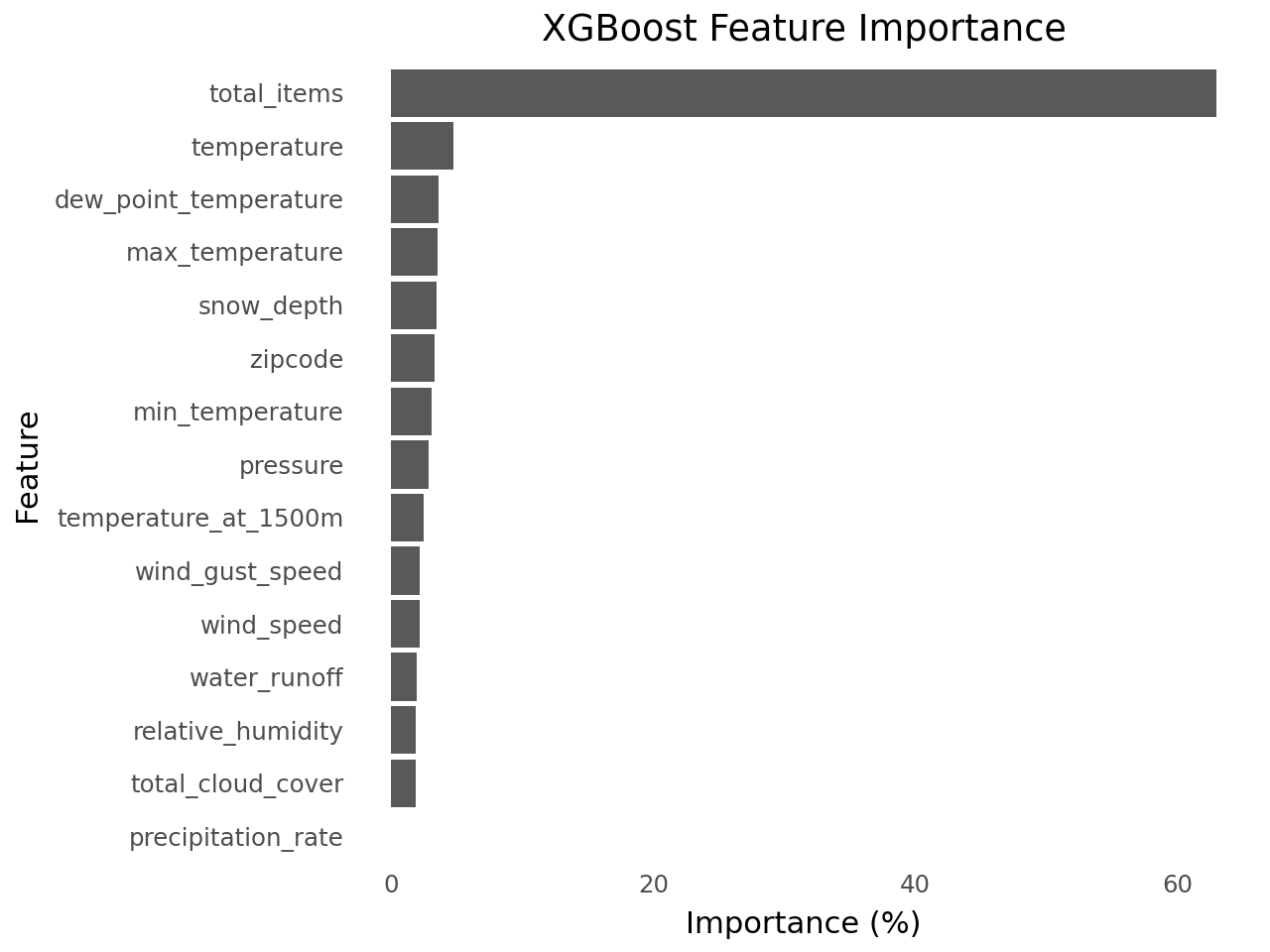
Check Feature Importance¶

importances = xgb_model.feature_importances_
features = X.columns

df_feat_imp = pd.Series(importances, index=features).sort_values().reset_index()

df_feat_imp.columns = ["feature", "importance"]
df_feat_imp["importance_pct"] = df_feat_imp["importance"] * 100

df_feat_imp

Loading...

from plotnine import (
    ggplot,
    aes,
    geom_col,
    coord_flip,
    labs,
    theme_minimal,
    theme,
    element_blank,
)

(
    ggplot(df_feat_imp, aes(x="reorder(feature, importance_pct)", y="importance_pct"))
    + geom_col()
    + coord_flip()
    + labs(title="XGBoost Feature Importance", x="Feature", y="Importance (%)")
    + theme_minimal()
    + theme(panel_grid_major=element_blank(), panel_grid_minor=element_blank())
)

<plotnine.ggplot.ggplot object at 0x00000188DB567E30>

Why does "total_items" have such high feature importance?

One surprising result from the gradient-boosted model was that the variable "total_items" accounts for nearly 63% of total feature importance.

At first glance, this may seem unusually high. However, there are several possible explanations.

From a logistics perspective, the number of items in an order can strongly influence delivery performance:

More items may require longer picking and packing time.
Larger orders may require larger or heavier packaging.
Complex orders increase warehouse handling complexity.
Bulk orders may experience fulfillment bottlenecks during peak periods.

It is important to distinguish between:

Predictive importance (useful for forecasting), and
Causal influence (driving the outcome).

Even if "total_items" is highly predictive, it does not necessarily mean that increasing the number of items directly causes delays. It may be:

A proxy for order complexity,
A proxy for warehouse congestion,
A signal of high-demand periods,
Correlated with geographic or seasonal patterns.

Models detect patterns, not causal mechanisms.